in a homogeneous isotropic medium at
equilibrium, with no source terms present and an obstacle
 compute the
acoustic field scattered by the obstacle when hit by the incoming
wave.
C. Dionisi , F. Mariani , M. C. Recchioni , F. Zirilli
We study two mathematical models concerning two applications taken from science and engineering. The mathematical models have been solved using highly parallelizable
numerical methods. These numerical methods have been implemented on the ENEA Grid using
distributed computing through the JOB ARRAY instruction of LSF.The
first application (acoustic obstacle scattering) uses also parallel
computing through the message passing library MPI.
The science application concerns acoustic obstacle scattering, the engineering application concerns cascading blackouts in a power transmission network.
Warning: If your browser does not allow you to see the content of this website click here to download a pdf file that reproduces the material contained here.
1. Acoustic obstacle scattering
We consider the following problem [1], [2], [3]:
Given an acoustic
incoming plane wave, not necessarily time harmonic propagating, with
wave propagation velocity
in a homogeneous isotropic medium at
equilibrium, with no source terms present and an obstacle
compute the
acoustic field scattered by the obstacle when hit by the incoming
wave.
The obstacle is assumed to be a bounded simply connected open
set with locally Lipschitz boundary
 contained in the three
dimensional Euclidean space and to be characterized by a constant
acoustic boundary impedance
 .
The incoming wave
 ,
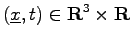 is assumed to satisfy the
wave equation (1) in
 .
The obstacle
 when hit by the incoming wave
,
generates a scattered wave
 ,
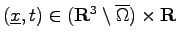 solution of the following exterior problem for the wave equation:
 is given by:
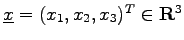 , the superscript
 means transposed,
 ,
 ,
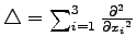 is
the Laplace operator,
is the wave propagation velocity and
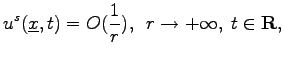
 and
 are the Landau symbols. An obstacle
 that when hit by the incoming wave
 generates
a scattered wave
 solution of (1)-(5)
sometime is called passive obstacle.
The algorithm proposed to solve (1)-(5) is a generalization of the ``operator expansion method'' developed in [1] and it reformulates the exterior problem for the wave equation using a perturbation approach. More specifically the algorithm proposed assumes that the incoming wave and the scattered wave can be represented as a superposition of time harmonic plane waves and reduces the solution of the time dependent problem for the wave equation to the solution of a set of time harmonic scattering problems, that is to the solution of a set of exterior boundary value problems for the Helmholtz equation, one problem for each frequency in the spectrum of the incoming wave.
Next we assume that the space dependent part of the solution of each
time harmonic problem for the Helmholtz equation can be
represented as a single layer potential with a density (that must be
determined) defined on the boundary of a suitable obstacle  contained in
. The algorithm reduces the solution of each
exterior boundary value problem for the Helmholtz equation to the
solution of a set of integral equations defined on the boundary of
and of a ``reference'' obstacle
 .
The numerical
difficulty of these exterior problems can be measured using the
parameter  defined as the ratio between the characteristic
dimension of the obstacle and the wavelength of the time harmonic
component of the acoustic incoming wave considered. The parameter
is an a-dimensional quantity and large values of
correspond to high frequency scattering, that is to numerically
difficult problems.
In the numerical experiments presented in [1],
[2], [3], the ratios
considered range
in the interval [3,100]. This implies the use of high dimensional
vector spaces to approximate satisfactorily the corresponding systems
of integral equations. That is each system of integral equations in
the sequence mentioned above after being discretized to be solved
numerically becomes a large system of linear equations.
Represented on a generic base the matrices that approximate the
integral operators after the discretization will be dense matrices. The solution of large dense linear systems will become computationally (computing time and memory requirements) unaffordable even for moderate values of
.
A new way of using the wavelet transform and new bases of wavelets have been introduced and a version of the operator expansion method that constructs directly element by element the coefficient matrix of the sparse linear systems that approximate in the wavelet basis considered the systems of integral equations has been developed.
The resulting numerical method has been implemented on the ENEA
Grid [4] and is able to deal with realistic acoustic scattering problems
solving large (sparse) linear systems (up to approximately
 (real)) unknowns and equations.
These results are obtained running simultaneously clusters of 500 jobs on the ENEA Grid. The computation of the elements of the coefficient matrices of the linear systems considered and several other aspects of the numerical algorithm proposed can be carried out independently one from the other allowing the development of an efficient solver for exterior boundary value problems for the Helmholtz equation, particularly suited to be executed on a computing grid using distributed computing. The solution of the resulting sparse linear systems is done using parallel computing on the parallel machines present in the ENEA Grid.
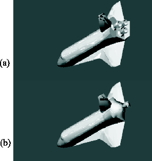
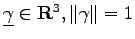
Several numerical experiments involving a simplified version of the NASA space shuttle (see Figure 1(b)) and incoming wave packets of the form:
 and
 , have been performed (see [3]).
The original model of the NASA space shuttle shown in Figure
1(a) has been modified to obtain the simplified model of
the NASA space shuttle shown in Figure 1(b). This
simplification is necessary in order to represent using a single
valued function the boundary of the obstacle in cylindrical
coordinates. This last fact makes easy the implementation of the operator expansion method. The data relative to the original obstacle, Figure
1(a), are downloadable from the website http://avalon.viewpoint.com/. The reference surface
 and the internal surface
 have
been obtained manipulating the 3D model shown in Figure
1(b).
We note that the physical dimensions of the shuttle are
expressed in  where
 =

 . The
maximum length of the shuttle model shown in Figure 1(b)
is of
 in the direction of the symmetry axis of its main
body. This symmetry axis has been chosen as cylindrical axis (
 -axis) of the
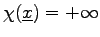
cylindrical coordinate system. Moreover we consider an acoustically
hard space shuttle that is
 ,
 and we recall that the sound speed in the air is

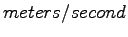 that corresponds to

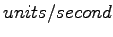 .
The ratio
of the boundary value problems for the Helmholtz equation considered in these experiments ranges from
a few tens to about one hundred.
Several animations and virtual reality applications concerning the numerical experiments discussed here and in [3] are shown in the website www.econ.univpm.it/recchioni/scattering/w12/A more general reference to the work of some of the authors and of their coauthors in numerical scattering is the website www.econ.univpm.it/recchioni/scattering.
2. Cascading blackouts in a power transmission network
In the last years the frequent and sometimes impressive current breaks registered around the world made urgent the problem of understanding the behaviour of the high voltage power transmission networks in critical conditions in order to characterize adequate operations to protect their functions. Unfortunately the structural complexity of the real power transmission networks, due to the high dependence between the components of the network, complicates the study of their behaviour and is the main cause of their vulnerability. In fact, due to this interdependence, local overloads of lines or local failures of components can generate cascades of current breaks that, in extreme cases, can cause the fall of the whole network. We name this phenomenon: ``cascading blackout''.
The blackout can be caused by inefficiency of the power transmission network or by excessive electric current demand from the loads that exceeds the network capacity. The cascading blackout is a sequence of events characterized by line failures and/or load sheds.
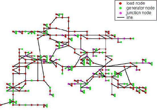
We represent a power transmission network as an undirected graph, that is as a set of nodes connected by branches. The nodes can be classified in three categories: generator nodes, representing wirings generating electricity, load nodes, constituting the load of the network, and junction nodes. The branches connecting the nodes represent the network transmission lines where the electric power flows. The lines have their own characteristic admittance, small values of the admittance correspond to small power flow through the lines.
Let  be the number of nodes in the network considered and for
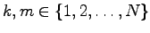 let
 be the line connecting the node
 to the node
 , in order to describe the electric power flow in the network the following quantities are considered:
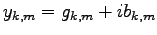 the admittance associated to the line
, where
 is the imaginary unit,
 and
 are, respectively, the conductance and the susceptance of the line
,
 the upper limit of the real power generated at the node k,
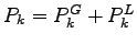 the active power injected into the node k, where
 e
 are, respectively, the real power generated and the real power demanded by the node k,
 the power flowing through the line
,
 the upper power flow limit of the line
,
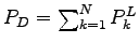 the total load power demand,
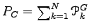 the total network capacity,
 the the complex voltage at node
.
Assuming assigned the network parameters mentioned above, in order to
represent the power flow through the network, we solve the DC (Direct
Current) optimal power flow problem, that consists in finding the
vectors
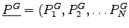 ) and the
corresponding voltage angles
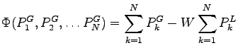
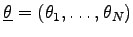 that minimize the following cost function:
subject to the constraints:
where W is a real positive constant representing a cost associated to the load nodes (we choose W=100).
The optimal DC power flow model, describes the network behaviour in
steady state regime when the values of the parameters characterizing
the model (the load power vector
 , the generators and
the lines capacities, the modulus of the generators voltages and the lines
admittances) are assigned.
Changes in the parameter values vary the network behaviour eventually
causing blackouts. We simulate the cascading blackout dynamics as a
consequence of variations of the total load power demand  assuming assigned the values of the remaining parameters.
As the total load power demand
grows, the solution of the
optimal DC power flow problem goes through some changes. The blackout
happens when the DC optimal power flow problem (7)-(9) becomes unfeasible. In
this case it is necessary to shed loads and/or to disconnect lines in
the attempt of restoring feasibility of the model and in this way a
new problem is formulated. If the new problem is also unfeasible, we
continue to disconnect lines and/or to shed loads following some
simple rules specified in [5] until we find a feasible problem and
finally we solve the resulting feasible problem. This sequence of
events generates the blackout cascade and mathematically corresponds
to the formulation and the solution of a sequence of constrained
optimization DC problems. That is we simulate with a numerical scheme
the sequence of events that generates a cascading blackout.
We consider as blackout size measure the quantity:
 where
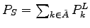 , and
 denotes the subset of
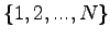 that contains the indices corresponding to the loads shed as a consequence of the blackout cascade.
We have
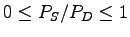 (the maximum value
 corresponds to total blackout).
Moreover in order to study the phase
transition phenomenon in the network from a statistical point of view
we analyze the network behaviour when the load power demand vector
 is subject to random fluctuations.
Starting from a reference value of the load power vector
we overload the network adding to the components of
a random disturbance, that is we change the value of the total
power demand
of a random quantity. As a consequence of that the
resulting blackout size measure
becomes a random variable
and we compute an approximation of its probability density function (pdf).
The analysis points out the existence of two values of the mean total
power demand  ,
 , with
 , of
the mean total power demand
such that the blackout size measure
probability density function corresponding to values
 is best fitted by a negative exponential function of
and the
blackout size measure probability density function corresponding to
values
 is best fitted by an inverse power function of
. This phenomenon is reminiscent of the phase transition phenomenon of equilibrium statistical mechanics. We note that the existence of the values
and
can be easily established numerically and that this is enough
to confirm the existence of the phase transition phenomenon.
The particular case of the Italian high voltage power transmission network (Figure 2) has been studied and the simulations needed to approximate the blackout size pdf have been obtained with a FORTRAN code running on the ENEA Grid. These simulations are run using distributed computing, that is running clusters of hundreds of independent jobs on the grid.
The Italian high voltage power transmission network is represented as
an undirected graph constituted of  nodes, with
 generator nodes,
 load nodes and
 junction nodes,
and
 lines. Note that we will consider junction nodes as load
nodes with power load smaller than
 . In this network
there are 14 lines that are double lines (i.e. there are two lines
joining the same two nodes). We substitute the double lines joining
the corresponding nodes with a single line whose admittance is given
by the sum of the admittances of the lines constituting the double
line. Therefore the total number of lines in the network that we study
is equal to
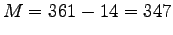 (see Figure 2).
The numerical simulation of the network behaviour shows that the interval
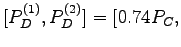
![$ 0.77 P_C]$](img99.png) can be chosen as critical interval.
Finally we study the line occupation.
For
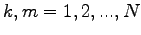 , we define occupation of the line
the
value
 when
 , when
 the occupation of the line is not considered, in fact
in this case the branch
of the graph does not represent a
real transmission line of the network. When we consider a sample of
power flows on a network we can compute the mean values of the line
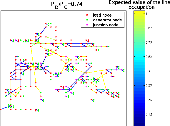
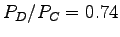
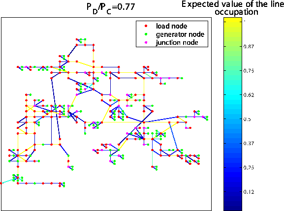
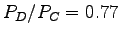
occupations of the sample. Figures 3 and 4 show for each line the expected value of the line occupation (on a sample of 20000
simulations) when
 takes the critical values
 and
 .
We can see that, in general, the line occupation is not homogeneous, that is the occupation of some lines is considerably greater than the occupation of the remaining lines of the network. This unbalance between line occupations can be the origin of large blackouts even when the mean value of the total power demand is smaller than the total network capacity. Note that the majority of the very loaded lines in Figures 3, 4, that is the lines whose occupation is close to one (the yellow lines in the figures), coincide. This fact suggests that these lines are the most vulnerable lines of the high voltage power transmission network considered in this study case.
The website http://www.ceri.uniroma1.it/ceri/zirilli/w1 contains some auxiliary material including animations that helps the understanding of the phenomena studied.
References
[1] M. C. Recchioni and F. Zirilli, The use of wavelets in the operator expansion method for time dependent acoustic obstacle scattering, SIAM J. Sci. Comput., 25, (2003), pp. 1158-1186.
[2] S. Migliori, G. Bracco, L. Fatone, M. C. Recchioni and F. Zirilli, A parallel code for time dependent acoustic scattering involving passive or smart obstacles submitted to The International Journal of High Performance Parallel Computing and Applications.
[3] L. Fatone, G. Rao, M. C. Recchioni, F. Zirilli, High performance algorithms based on a new wavelet expansion for time dependent acoustic obstacle scattering, Communications in Computational Physics, 2(6), (2007), pp. 1139-1173.
[4] S. Migliori, G. Bracco, C. Dionisi, F. Mariani, M. C. Recchioni, F. Zirilli, Parameter choice models for two codes running on the ENEA grid , Report ENEA, 2007
[5] A. Farina, A. Graziano, F. Mariani, F. Zirilli, Probabilistic analysis of failures in power transmission networks and ``phase transitions'': a study case of an high voltage power transmission network, to appear in Journal of Optimization Theory and its Applications.